Before lunch, I posted on a new phytools function, threshBayes, in which we can use Bayesian MCMC to sample evolutionary model parameters & liabilities on the phylogeny from their joint posterior distribution using MCMC. For more information on the threshold model in phylogenetics, see Felsenstein (2005, 2012) and my previous post. Here, I'm going to illustrate simulation & estimation under this model using phytools & threshBayes in R.
OK, first let's simulate a pure-birth phylogeny for (say) 200 species. We can also simulate our so-called liabilities up the tree with a correlation of 0.8:
> # load phytools & source
> library(phytools)
> source("threshBayes.R")
> # simulate
> tree<-pbtree(n=200,scale=1) # tree
> Xl<-sim.corrs(tree,vcv=matrix(c(1,0.8*sqrt(2),0.8*sqrt(2),2), 2,2)) # liabilities
Now, we can substitute one of these characters (say, trait 1) for a binary trait evolved under the threshold model, setting the threshold to +-0.
> X<-Xl
> X[Xl[,1]<0,1]<-0
> X[Xl[,1]>0,1]<-1
> X
[,1] [,2]
t1 0 -0.05615011
t2 1 0.42579821
t3 1 -0.32314924
t4 0 . . .
Now we are ready to run our MCMC. We'll just use the default control parameters and priors. Note that this may take some time - certainly at least several minutes even on a fast computer.
> mcmc<-threshBayes(tree,X,types=c("discrete","continuous"), ngen=500000)
[1] "gen 1000"
[1] "gen 2000"
[1] "gen 3000"
[1] . . .
The object returned by threshBayes is a list containing the posterior sample for the parameters of the evolutionary model and the liabilities at the tips. Note that for a continuous character liabilities are not sampled (they are treated as known), but these are still given in the posterior sample matrix. Also - we fix the rate of evolution at 1.0 for the liability of our discrete character. This is because don't actually have any information about the scale of our underlying liabilities, and the probability of switching back and forth between states on either side of the threshold is independent of the Brownian rate of evolution of liability (this is probably better explained in Felsenstein 2012).
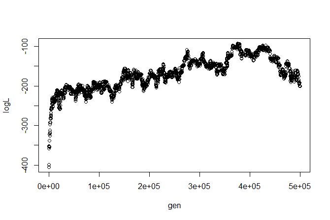
We can, say, plot the likelihood profile:
I'm not sure how I feel about this likelihood profile (we might want to change our proposals or run multiple chains), but let's ignore these issues for illustrative purposes. (Remember, we can always run all the traditional MCMC diagnostics using, say, 'coda.')
Let's cut off the first half of our posterior sample and get parameter estimates from the second 250,000 generations (2500 samples, in this case):
> estimates<-colMeans(mcmc$par[2501:nrow(mcmc$par),2:6])
> estimates
sig1 sig2 a1 a2 r
1.0000000 2.0309112 0.6746904 1.1889742 0.8341032
These are really close to the generating parameters (particularly for σ2 and r). To be fair, this was part of my motivation in using a "large" tree of 200 taxa, even though run time is considerably longer. Parameter estimates from the posterior sample were not nearly as close on smaller trees.
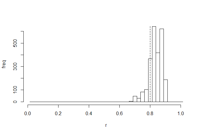
We are probably most interested in the correlation coefficient - so let's look at the posterior sample for this parameter, with the generating value (0.8, in this case), overlain as a vertical dashed line:
> h<-hist(mcmc$par[2501:nrow(mcmc$par),"r"],0:40/40+0.0125, main=NULL,ylab="freq",xlab="r")
> lines(c(0.8,0.8),c(0,max(h$counts)),lty="dashed")
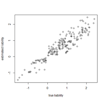
Finally, let's look at how close our true liabilities line up with estimates obtained by averaging the posterior sample:
> estLiab<-matrix(colMeans(mcmc$liab[2501:nrow(mcmc$liab), 1:200+1]),200,2)
> cor(Xl[,1],estLiab[,1])
[1] 0.9255481
> plot(Xl[,1],estLiab[,1],xlab="true liability",ylab="estimated liability")
Awesome. In this case, the generating & estimated liabilities match very well. Note that the estimated liabilities are scaleless - so although in this case they match well numerically, this is because we generated the liabilities under σ(liability)2=1.0. If we had instead simulated liabilities under a model of, say, σ(liability)2=100 or σ(liability)2=1000, then we would expect the correlation to be equivalent, but the liabilities themselves would not be as well matched numerically. Cool.
Next up - multiple states for the discrete character!


No comments:
Post a Comment
Note: due to the very large amount of spam, all comments are now automatically submitted for moderation.